Being a mature student

It felt like the planets aligned for me in perfect orientation. It was the start of September and the job I’d been doing for a year came to an abrupt end. I didn’t know what to do next: I had been toying with the idea of a distance learning degree through the Open University, but the thought of six years studying didn’t appeal.

A brief telephone conversation with the University of Brighton’s admissions team, and suddenly over the course of a few days I found myself enrolled on a full-time bachelor’s degree course. Still in a state of shock, three weeks later I am sat in a lecture hall listening to the Vice Chancellor welcoming me and my fellow ‘freshers’ to the University of Brighton. Wow!

Even now at the end of three years of study it still feels a little bit surreal. I have loved every minute of it, but as a mature student (and single parent) it is a very different journey to most of the students you share lecture halls and laboratories with.

In a strange twist, my son and I began university courses at different institutions in the same week. He studied International Politics at Aberystwyth University, whilst I studied Earth & Ocean Science at Brighton. This gave me a unique insight in to the process he was going through, but also meant my fellow students were the exact same age as my own child.

Of the approximately 300 students in the School of Environment and Technology for our year group, I was the only one over 25 (and nearly double that age at that!) My fellow students were an amazing bunch of people, who I loved working and studying with, but the generational gap was ever present.

The teaching and support staff at the University of Brighton do an amazing job under increasingly difficult circumstances. On one hand you have a student body that struggles to turn up on time, and when they do: turn up 20, 30, 40 minutes late for a lecture; think nothing of walking to the front of the lecture room; noisily empty their bag; talk to their friends; and generally disturb the rest of the room, whilst encased in a shroud of their own self-importance and oblivious awareness of the disruption they are causing. I am neither religious or violent, but at those moments I was praying for the god Nemesis to perform her primary role and administer divine retribution on the moron interrupting my learning.

I felt true sympathy for the teaching and support staff at the University, battling unforgivable student behaviour on one side, whilst being undermined, undervalued and overworked by the University administration on the other. Like so many parts of the education system in the UK, the University system is now a profit-making business ran by accountants with academic excellence and research a very poor and distant second place.

Everything from the quality, ethos and work ethic of my fellow pupils, to the workload and pressures on the teaching staff describes a system where the only thing that counts is the numbers enrolled on a course, that are subsequently paying £9000+ each year each.

I need to make it very clear I am not attacking any individual within the contact staff at the University, they are individuals who are passionate and determined to do the best they can, but they are working within a system that rewards quantity over quality.

On a personal note, I need to say a huge personal thank you to the following people who have made my undergraduate experience a life changing, exhilarating and thoroughly enjoyable experience.

Dr P Teasdale                                 Dr Norman Moles

Dr Jake Ciborowski                        Pete Lyons

Magda Grove                                 Dr Chris Carey

Dr Corina Ciocan                           Prof Chris Joyce

Prof David Nash                            Dr Annie Ockelford

Dr Ray Ward                     (apologies to anyone I missed off.)

When I enrolled as an undergraduate at the age of 47, I was already a little bit odd. Having worked well-paid jobs, and been completely unsatisfied with them, I had made the decision that personal fulfilment rather than financial gain would be my main motivator. But, as a single parent of two amazing children, and being their only financial support, it was only through their love and support that I could take us all through the arduous journey of undergraduate life in a society that does not respect education for its own sake, rather than as a tool to earn more money.

To my children Paige and Taylor, I can never thank you enough for your unwavering support.

Another thank you goes out to Heather, a very good friend who was always happy to help with my dissertation, in the sample collection process, regardless of the weather. She was always there to let me discuss findings and developments in my dissertation project, and most importantly was there to give me a kick up the arse when I thought I wasn’t good enough to do the work, when I doubted myself, or when I was just sick of the workload. Thank you.


To anyone thinking of going to University as a mature student, I would say unequivocally ‘do it’, you will never regret it, not for one second.

However…. be prepared to feel isolated in a system that is geared up for kids fresh out of the Higher education system.

Dissertation findings.

Now that the sampling, lab work and project writeup is all finished, I have detailed below some of my key findings and interpretations of the data. As has been mentioned in previous blog pieces, the biggest single finding from my research has been the paucity of data relating to the processes at play within the Adur Estuary, and how much more research is needed.

So what did I find?

Suspended sediment concentrations (SSC) within the samples were quite consistent across all samples collected. In the end, I collected ten full sets of samples across the three transects, five during Spring tides, and five during neap tides.

I also collected two sets of samples from a single location across an entire tidal cycle. Whilst sitting in the middle of the estuary for 13 hours may not be everyone’s idea of fun, the results I gained from these two data sets (again from both Spring and Neap tides) was really interesting.

The first thing to say about SSC from all twelve data sets is that they are incredibly low. Research conducted in macro tidal estuaries suggested SSC levels should have been in the range of 1000 to 10,000 ppm. The difference in tide heights between high and low water (tidal range) means that there is lots of energy in the water as it flows into and out of the estuary, thus enabling larger quantities of SSC to be present.

My findings for the Adur estuary showed typical results of around 30ppm, an incredibly low figure for a macro tidal estuary.

I would imagine that initial reactions to this will be surprise and relief, after all less SSC means less dredging and restriction to shipping channels. However, it would also mean less sediment available to the salt marshes and mud banks within the estuary to maintain their heights in a world of rising sea levels though.

The type of sediment carried within the water column is very interesting too. Analysis of the sediment contained within the samples, by passing it through a Laser Particle Size Analyser (LPSA) shows that the majority of SSC are silts and clays, with a surprisingly small amount of sand size particles contained within the water column.

LPSA results

The further right on the table the larger the grain size of the SSC gets. The red line demonstrates SSC at the mouth of the river, showing a small increase in sand sized grains.


The closer to open water samples were collected, so the concentration of sand size particles increased, but even as far downstream as the RNLI slipway, concentrations of sand particles were very low (<30% by volume).

This lack of sand size particles would perhaps suggest minimal marine sediment intrusion, or a much lower than expected energy regime within the estuary meaning the larger sand particles just cannot be picked up and carried by the water flow.

Data sets produced from a complete tidal cycle show a clearly defined and significant increase in SSC during the middle to later sections of the ebb tide. These spikes in SSC were almost identical during both Spring and Neap tides, also, high water slack tide and the flood tide both showed very reduced SSC levels.

SSC concentrations over an entire tidal cycle, with peak SSC values during the later stages of the ebb tide.


These results show that the estuary is an ebb tide dominated regime, with the falling tide being the period during which entrainment of sediment and its transportation within the estuary is at its greatest. These results imply that the Adur estuary is an asymmetrical tidal regime, with the flood tide occurring quickly, followed by a much more extended ebb tide due to the constricted shape of the estuary which extends ~8km inland. This long thin shape of the estuary (exacerbated by modern seawalls and flood defences) means that the retreating tide produces a ‘log jam’ effect upstream and causes the strength and period of the ebb tide to become extended.

These findings need much more empirical research to confirm, but personal anecdotal evidence of the delay between high tide at the estuary mouth and the beginning of the ebb tide upstream from Bramber supports the asymmetrical hypothesis. I found a delay of ~2 hours before the tidal flood waters started to recede after the tide table declaration of when it should have begun.

A Map showing the survey location and the confined but extended length of the river influenced by the tides.

My Dissertation on the Adur Estuary is finished.

It has felt like a long time coming, but my undergraduate dissertation project is finally finished and submitted. After months of collecting samples, analysis in the lab, and then pondering and considering the results, I feel like I finally start to understand the Adur Estuary a little bit better.

The biggest single realisation after over a year’s work is how much more research is needed to fully understand the estuary and the processes underway there:

  • Accurate and detailed logging of the tidal regime within the estuary and it’s changing dynamics dependant upon the tidal range are needed.
  • The impact the turbidity maximum has on the estuary and the suspended sediment concentrations (SSC), and how the turbidity maximum migrates along the estuary during the tidal cycle.
  • How do SSC from upstream, beyond tidal influences, differ to estuarine waters, and how will recent changes to sea defences change the estuary.

Considering the economic, social, and aesthetic importance of the Adur estuary to the larger area I am amazed how little research has been done into the characteristics and behaviour of the estuary. As a society we are happy to spend millions of pounds on defences, sea walls and protection measures, but do we truly understand the consequences of these changes?

The river Adur channel is highly constricted as it approaches the sea, and abstraction of water from the river seems to be at unprecedented levels and only increasing. Environment Agency data from Beeding Bridge at Bramber shows that freshwater discharge has dropped significantly three times in the last six years (Figure 1), with typical river levels dropping by 30% in just six years. This is at a time when rainfall levels for the South East of England are higher than historical levels, with the last three years (2015-2018) being 105% of the average for the last 100 years.

Figure 1. Freshwater discharge flow in the River Adur, West Sussex. With the black circles highlighting dramatic reductions in flow volumes.


So, less water is coming down the river even though more rainfall is falling within the Adur’s catchment.

Why should we care?

Freshwater discharge within the Adur can be seen to have two crucial roles:

1) it helps to bring sediment from upstream down the river (along with nutrients and phosphates from agricultural run-off) thus helping to supplement areas suffering coastal erosion, and help the accretion of areas being inundated by sea level rise (particularly salt marshes and mud flats, both essential habitats);

2) high discharge rates help to flush sediment through the estuaries navigable channels, keeping these working corridors operational, and producing net outflow of sediment into the marine environment, rather than net inflow and ingress of sediment from the sea.

The exact impact of changes to freshwater discharge in the Adur, and in macro-tidal estuaries generally, is still unclear. Our growing demand for freshwater, both for agriculture and as potable water is only going to increase. Should this be at the expense of our estuarine environments?

Filtering out suspended sediment.


Cuckmere Haven


Situated east of Brighton on the south coast of England, Cuckmere Haven sits in the midst of the iconic chalk cliffs and the South Downs national park. The Cuckmere valley is a stunning wetland environment that has salt marshes, saline lagoons, shallow wetlands, and wet grasslands.

But….. it is incredibly popular with tourists and locals alike, and to enjoy the stunning landscape fully I like to have it all to myself (almost anyway).

An early start (in May, that means up at 4AM) gets you to the Coastguard cottages car park just outside Seaford before Sunrise.

Image from Google Maps.

A short walk through the pre-dawn light brings you to the cliffs overlooking the sea and the Cuckmere estuary. It’s a beautiful and tranquil time, with the wildlife around you just waking up. Then comes the sunrise over the far side of the valley, and it looks like the hills are on fire. And the best thing of all is you get to revel in this majestic spectacle all by yourselves.

By this time it was about 5.45Am and this was the cue for the birds, rabbits, and insects to wake up fully. The quiet soon disappeared beneath a growing cacophony of bird song, and insect buzzing.


A truly beautiful place, and well worth the early start to the day.


All images are copyright S Hall.

Geohazard report – Tokyo.

Following the catastrophic earthquake and tsunami in Northeast Japan in March 2011, is Tokyo at greater risk of destruction?

Plate tectonics as a theory to explain earthquakes, volcanism and continental migration over geological timescales is a mature theory that has developed and been refined since Alfred Wegener first proposed his theory in 1912 (Wegener, 1966), through to the development of the theory in the 1970’s (Dickinson, 1974). The movement of these tectonic plates, and the subsequent frictions in the upper 10 to 15 KM between them is the principle cause of energy release which manifests itself in the form of earthquakes and sudden displacement of large sections of these plates. Below the upper crust boundary (10 to 15 Km depth) the crust accommodates plate movements through ductile deformation, whilst elastic-brittle characteristics are dominant in the upper crust, thus most earthquakes originate from depths less than 15 Km (Maggi et al, 2000).

The friction between the boundaries of two joining tectonic plates and the speed of plate movement dictates the frequency and magnitude of the plate movement when it occurs (Lachenbruch, 1980). In a low friction environment frequent lower magnitude quakes can be a sign that energy is being released, thus preventing the accumulation and subsequent release of larger magnitude events (Kanamori and Anderson, 1975).

Release of energy in the form of earthquakes causes earth movement and shaking, but if the event occurs within a subaqueous setting, and there is either a substantial movement of seabed either in the form of plate thrust and uplift, or a major seafloor avalanche then the sudden displacement of large amounts of water can cause a tsunami (Song et al, 2017).

Tsunamis can travel through deep waters such as found in the open Pacific at tremendous speeds, and as experienced in the ‘boxing day tsunami’ of 2004 (Farrell et al, 2015), coastal areas physically remote from the location of the earthquake can be dramatically and devastatingly affected. Because of the remote nature of tsunami threats, the extensive seismic activity surrounding the north Pacific coastlines of East Asia and North America, the so called ‘ring of fire’, means the threat of a tsunami source is extensive (Kânoğlu and Synolakis, 2015).

Japan sits to the West of a number of major subduction zones, with the Pacific plate subducting beneath the Okhotsk plate, as well as the Philippine plate subducting beneath the Amuria and Okhotsk plates (Figure 1) (Schellart et al, 2011). The rate of plate movement in this region is amongst the highest in the world (Figure 2), with Tokyo itself being located on the Okhotsk plate and very close to all other plates’ subduction margins mentioned above (Uchida et al, 2016).

1

Figure 1. Map showing the tectonic plate configuration surrounding Japan. Plate movement direction (large red arrows) and subduction zones (red lines) marked. Also marked is the focal point of the 11 March 2011 earthquake and tsunami.

Source: Ozawa et al, 2011.

2

Figure 2. Global tectonic plate boundaries with plate movement direction shown by green arrows, blue arrows indicate the rate of subduction, and red arrows indicate the rate of trench migration.

Source: Schellart et al, 2011:Figure 2.


Due to the regions extensive and frequent experiencing of seismic activity, the Japanese have rigorous building control measures in place (Imamura et al, 2018), as well as public awareness programs (Esteban et al, 2018) and sea defences in preparation for earthquakes and subsequent tsunamis (Suppasri et al, 2016). The magnitude of the event is key however in deciding the degree of preparation required. The last decade alone has seen 15,343 earthquakes in and around Japan between 3.5 and 7.5 magnitude event (See figure 3 for area parameters: USGS, 2018), with 124 events in the last 100 years ranging from 7 to 7.9 magnitude (Figure 3) (United states geological survey, 2018).

3

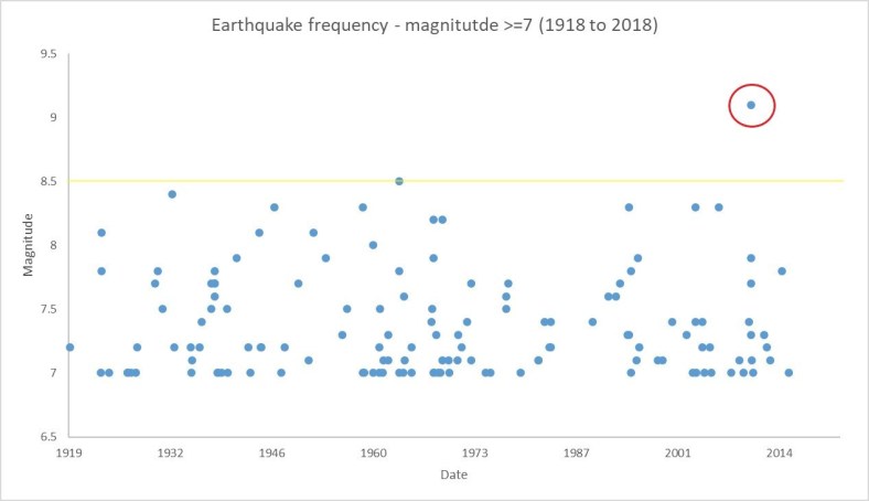
Figure 3. Earthquakes occurring near to Japan in the last 100 years equal to or above magnitude 7 intensity. Yellow line indicates highest previously recorded event of 8.5 magnitude, with the red circle highlighting the 11 March 2011 event of magnitude 9.1.

Source https://earthquake.usgs.gov/earthquakes/ (Area parameters used 47.142° (N), 25.618° (S), 120.85° (W), 152.93° (E).

Hazards arising from any earthquake event can be separated in to two key areas; earthquake related hazards such as liquefaction, landslip/landslides, ground shaking, and ground rupture; and tsunami hazards from land inundation by catastrophic volumes of water displaced by seafloor movement, directly related to the earthquake (Dunn et al, 2012). The magnitude of the 2011 event has meant that legislation, preparation and mitigation of future seismic events now incorporate the expectation and possibility of megathrust earthquakes happening (Santiago-Fandino et al, 2017).

11th March 2011 saw one of the largest earthquake in recorded history to strike Japan, registering as a magnitude 9.0 event (Ozawa et al, 2011; Hooper et al, 2013). 15,896 people lost their lives, with a further 8,694 people either injured or reported missing (National Police Agency of japan, 2018). Economic losses to the Japanese economy were estimated to be up to US$235 Billion (World Bank, 2011), with the damage to infrastructure and particularly the nuclear installation at Fukushima Daiichi causing an estimated 59,000 people still unable to return to their homes as of January 2016 (Japan Times, 2016).

Occurring at 14:46 JST (Japanese standard time), the oceanic megathrust earthquake was located 70 kilometres east of the Oshika Peninsula, rupturing an extended section of the fault plane ~500Km long (Suzuki et al, 2011; United States Geological Survey, 2016). A megathrust earthquake is one of the most destructive magnitude earthquake events (usually >9 magnitude) and is differentiated from other earthquakes by its intensity and potential to generate very large tsunami waves (Biley and Lay, 2018). The elastic energy retained within the Okhotsk Plate, generated by the frictional force of the subducting Pacific Plate passing beneath it, was dramatically and explosively released. The damage from the earthquake was then followed by a tsunami as the significant movement of the seafloor (~62m movement) displaced massive volumes of seawater (Sun et al, 2017). This reached up to 40m high tsunami waves as the waters reached the Japanese shoreline and inundated the coastal regions by up to 10 Km inland (Mori, 2011).

Whilst the megathrust earthquake was expected (Davis et al, 2012), the predicted 8 to 8.6 magnitude force prediction was significantly underestimated. As seen in figure 3 though, the unprecedented magnitude of the 2011 earthquake in comparison to the previous 100-year record demonstrates the extreme nature of the scale of the event. Research since the 2011 event is now incorporating historical data such as geological evidence in the form of previous tsunami deposits within coastal stratigraphy (Wallis et al, 2018) and historical records which are extensive in Japan which detail tsunami damage and deaths dating back millennia (Ouzounov et al, 2018).

Seismic monitoring in the North West Pacific region is some of the most detailed and extensive in the world (Huang et al, 2017), but as demonstrated in the 2004 Boxing Day tsunami which affected the Indian Ocean originating off the Western coast of Northern Sumatra (Lay et al, 2005), travel distances of tsunami waves can be global with deaths and damage being inflicted ~8000 Km away in Cape Town, South Africa (Mail and Guardian, 2004). This extensive range of the impact of a megathrust earthquake in the form of a tsunami means that extensive parts of ‘the ring of fire’ perimeter of the Pacific could be the origin of a tsunami that could affect Japan (Hinga, 2015). So, although the 2011 event has dissipated some energy in this particular length of plate boundary through the earthquake, tensional increases in plate boundaries adjoining the affected area may have been increased (Toda et al, 1998) including plate margins close to Tokyo, Japan’s capital. This increase in potential fault stress raises the risk of tsunami sources originating close to the Japanese coastline, a major factor in the intensity of wave height experienced in the 2011 event. Japan also must consider the possibility of other areas within the Pacific ‘ring of fire’ generating significant seismic events that could impact their shorelines in the form of tsunami waves.

With a population of 13.8 million people, and an extended metropolitan area encompassing over 38 million people (Tokyo Metropolitan Government Bureau of Statistics Department), Tokyo is the world’s most populous metropolitan area (UN, 2017). With population density of  up to 14,883 people/km2 within the cities prefecture (Statistics Bureau, 2018), hazards and the magnitude of the casualties would be compounded and exacerbated by the population levels present (Uitto, 1998). Population density of the Ibaraki-ken prefecture (one of the worst affected areas in the 2011 event) was just 485 people/km2, and even though casualty figures would not be directly proportionate, the resultant numbers of injured or dead would be extreme in an event affecting Tokyo.

Tokyo, Japan’s capital and largest urban conurbation, has additional unique factors which mean that seismic hazard events are incredibly difficult to predict, with the historic record showing three major earthquakes affecting Tokyo in 1703, 1855 and 1923 (Bozhurt et al, 2007). Immediately following the 2011 seismic event to the North of Tokyo, off the Oshika peninsular, a magnitude 7.9 event was recorded close to Japan just 30 minutes after the main earthquake (Simons et al, 2011). The scale of the 2011 event, and the proximity to the countries capital has meant that city impacting hazard models have had to be revised their potential maximum magnitude (Imamura et al, 2018).

Located at the juncture of three tectonic plates, Tokyo is located close to the Sagami trench, a zone in which the complex subduction may well limit the maximum magnitude of earthquake to hit (Toda et al, 2008). Below Tokyo, due to the interaction of two separately subducting plates, a complicated layering is potentially underway known as the Kanto fragment (Stein et al, 2006), causing frictional tensions at two separate boundaries and thus increasing the complexity of earthquake prediction (Figure 4).

4

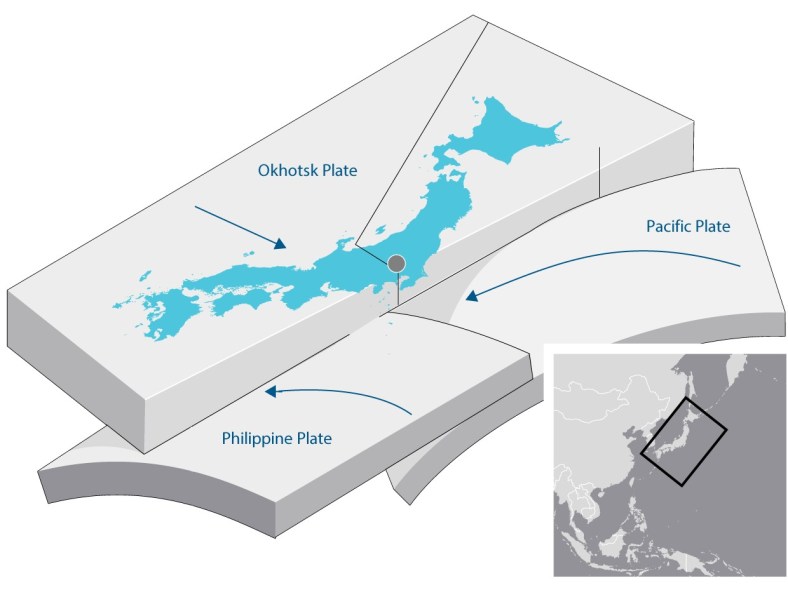
Figure 4. Stylised representation of the tectonic plate configuration caused by the subduction of both the Pacific and Philippine plates beneath the Okhotsk plate, and the layered configuration of the lithosphere. (Insert shows Japan in relation to the Western Pacific. Source: Modified from the Guardian Newspaper  https://www.theguardian.com/world/2015/may/31/japan-alert-powerful-earthquake


Topography considerations are also a major factor to consider for Tokyo’s tsunami risk, as the city sits at the North Western edge of Tokyo bay, a large shallow bay with a narrow 9 Km opening (Figure 5). Modelling of tsunami risks affecting Tokyo itself produce conflicting results with the narrow entrance to Tokyo Bay potentially protecting the city or amplifying tsunami damage (Sasaki et al, 2012) depending upon the magnitude and location of source used within models.

5

Figure 5. Stylised 3D map of Tokyo Bay and the surrounding bathymetry showing the constrained entrance to the bay. Source: Google maps.

Liquefaction hazards in Tokyo have been identified following the 2011 event by using Lidar surveying pre and post event (Konagai et al, 2012). This process has generated high resolution results to determine areas affected, and subsequently at future risk of soil subsidence (Figure 6) (Yasuda et al, 2012). Identification of risk allows remediation and prevention works to be undertaken to prevent future earthquake damage due to liquefaction (Bhattacharya et al, 2011).

6


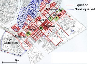
Figure 6. Example of areas within Tokyo mapped after the 2011 event, demonstrating liquefaction predominantly on reclaimed land. Source: Yasuda et al, 2012


Building codes (dictating earthquake resilience) were updated extensively in 1981 throughout Japan, dictating that buildings should be built to remain standing when affected by an earthquake of 7 magnitude or higher (Aoyama, 1981). This is a requirement of new buildings constructed after 1981, therefore buildings constructed prior to this date (known as Kyu-Taishin) have a potentially lower resilience to high magnitude earthquakes compared to those constructed post 1981 (known as Shin-Taishin) (Sharma and Louzado, 2015). Kyu-Taishin (older, less resilient buildings) constitute ~20 to 30% of buildings throughout Japan, and therefore continue to be a potential hazard source as demonstrated in the 1995 Hanshin earthquake where 8.4% of older buildings were seriously damaged, compared to 0.3% of Shin-Taishin (building constructed to the newer more stringent building regulations).

To answer the original question, as to whether Tokyo is at greater risk of destruction following the 2011 event, we need to define ’risk’. Disaster prediction and prevention defines risk as the hazard multiplied by vulnerability, divided by the resilience or ‘capacity to cope’ (Smith, 2003). In Tokyo’s current situation, it can be argued that the hazard of a megathrust event has been increased due to the changes in tension regime along the faults near to Tokyo (Stein, 1999). Awareness of this risk, and specifically a realisation of the scale of the potential magnitude of events, which may well exceed the maxima encountered within recorded history, enables relevant bodies and individuals to be prepared. This ability to prepare and engineer for events far exceeding previously estimated maximum magnitudes can diminish the vulnerability of those within the affected area, as well as increasing the resilience and ability to cope with a major event (such as the 2011 event).

After considering all the evidence examined within this discussion, I feel even though the hazard from a megathrust event and subsequent tsunami may have increased since the 2011 event, raised awareness of the potential hazard may have diminished vulnerability and increased resilience, thus meaning risk has remained at the level prior to the 2011 event.


References

Aoyama, H., 1981. Outline of earthquake provisions in the recently revised Japanese building code. Bulletin of the New Zealand Society for Earthquake Engineering, 14(2).

Bhattacharya, S., Hyodo, M., Goda, K., Tazoh, T. and Taylor, C.A., 2011. Liquefaction of soil in the Tokyo Bay area from the 2011 Tohoku (Japan) earthquake. Soil Dynamics and Earthquake Engineering, 31(11), pp.1618-1628.

Bilek, S.L. and Lay, T., 2018. Subduction zone megathrust earthquakes. Geosphere, 14(4), pp.1468-1500.

Bozkurt, S.B., Stein, R.S. and Toda, S., 2007. Forecasting probabilistic seismic shaking for greater Tokyo from 400 years of intensity observations. Earthquake Spectra, 23(3), pp.525-546.

Davis, C., Keilis-Borok, V., Kossobokov, V. and Soloviev, A., 2012. Advance prediction of the March 11, 2011 Great East Japan Earthquake: A missed opportunity for disaster preparedness. International Journal of Disaster Risk Reduction, 1, pp.17-32.

Dickinson, W.R., 1974. Plate tectonics and sedimentation.

Dunn, C., Degg, M.R., Digby, B. & Warn, S. 2012, Tectonic hazards, Geographical Association, Sheffield.

Esteban, M., Bricker, J., Arce, R.S.C., Takagi, H., Yun, N., Chaiyapa, W., Sjoegren, A. and Shibayama, T., 2018. Tsunami awareness: a comparative assessment between Japan and the USA. Natural Hazards, pp.1-22.

Farrell, E.J., Ellis, J.T. and Hickey, K.R., 2015. Tsunami case studies. In Coastal and Marine Hazards, Risks, and Disasters (pp. 93-128).

Hinga, B.D.R., 2015. Ring of Fire: An Encyclopedia of the Pacific Rim’s Earthquakes, Tsunamis, and Volcanoes: An Encyclopedia of the Pacific Rim’s Earthquakes, Tsunamis, and Volcanoes. ABC-CLIO.

Hooper, A., Pietrzak, J., Simons, W., Cui, H., Riva, R., Naeije, M., van Scheltinga, A.T., Schrama, E., Stelling, G. and Socquet, A., 2013. Importance of horizontal seafloor motion on tsunami height for the 2011 Mw= 9.0 Tohoku-Oki earthquake. Earth and Planetary Science Letters, 361, pp.469-479.

Huang, P., Whitmore, P., Johnson, P., Bahng, B., Burgy, M., Cottingham, T., Gately, K., Goosby, S., Hale, D., Kim, Y.Y. and Langley, S., 2017, September. Real-time earthquake monitoring and tsunami warning operations at the US National Tsunami Warning Center. In OCEANS–Anchorage, 2017 (pp. 1-6). IEEE.

Imamura, F., Suppasri, A., Sato, S. and Yamashita, K., 2018. The Role of Tsunami Engineering in Building Resilient Communities and Issues to Be Improved After the GEJE. In The 2011 Japan Earthquake and Tsunami: Reconstruction and Restoration (pp. 435-448). Springer, Cham.

Japan times. 2018. The Japan Times. [Online]. [27 November 2018]. Available from: https://www.japantimes.co.jp/news/2016/03/07/national/social-issues/11-tohoku-disaster-displaced-remain-shelters-10-years-study-finds/

Kanamori, H. and Anderson, D.L., 1975. Theoretical basis of some empirical relations in seismology. Bulletin of the seismological society of America, 65(5), pp.1073-1095.

Kânoğlu, U. and Synolakis, C., 2015. Tsunami dynamics, forecasting, and mitigation. In Coastal and marine hazards, risks, and disasters (pp. 15-57).

Lachenbruch, A.H., 1980. Frictional heating, fluid pressure, and the resistance to fault motion. Journal of Geophysical Research: Solid Earth, 85(B11), pp.6097-6112.

Lay, T.; Kanamori, H.; Ammon, C.; Nettles, M.; Ward, S.; Aster, R.; Beck, S.; Bilek, S.; Brudzinski, M.; Butler, R.; DeShon, H.; Ekström, G.; Satake, K.; Sipkin, S. (20 May 2005). “The Great Sumatra-Andaman Earthquake of 26 December 2004”. Science. 308 (5725): 1127–1133

Maggi A. Jackson J. McKenzie D. Priestley K., 2000a. Earthquake focal depths, effective elastic thickness, and the strength of the continental lithosphere, Geology , 28, 495–498.

Mail and guardian. 2004. Mail and Guardian. [Online]. [3 December 2018]. Available from: https://mg.co.za/article/2004-12-28-4-south-africans-die-in-tsunami-disaster

Mori, N., Takahashi, T., Yasuda, T. and Yanagisawa, H., 2011. Survey of 2011 Tohoku earthquake tsunami inundation and run‐up. Geophysical research letters, 38(7).

National police agency of japan. 2018. Police countermeasures and damage situation associated with …. [Online]. [20 November 2018]. Available from: https://www.npa.go.jp/news/other/earthquake2011/pdf/higaijokyo_e.pdf

Ouzounov, D., Pulinets, S., Hattori, K. and Taylor, P., 2018. Pre-Earthquake Processes: A Multidisciplinary Approach to Earthquake Prediction Studies (Vol. 234). John Wiley & Sons.

Ozawa, S., Nishimura, T., Suito, H., Kobayashi, T., Tobita, M. and Imakiire, T., 2011. Coseismic and postseismic slip of the 2011 magnitude-9 Tohoku-Oki earthquake. Nature, 475(7356), p.373.

Santiago-Fandiño, V., Sato, S., Maki, N. and Iuchi, K. eds., 2017. The 2011 Japan Earthquake and Tsunami: Reconstruction and Restoration: Insights and Assessment After 5 Years (Vol. 47). Springer.

Sasaki, J., Ito, K., Suzuki, T., Wiyono, R.U.A., Oda, Y., Takayama, Y., Yokota, K., Furuta, A. and Takagi, H., 2012. Behavior of the 2011 Tohoku earthquake tsunami and resultant damage in Tokyo Bay. Coastal Engineering Journal, 54(01), p.1250012.

Schellart, W., Stegman, D., Farrington, R., and Moresi, L. (2011). Influence of lateral slab edge distance on plate velocity, trench velocity, and subduction partitioning. Journal of Geophysical Research. 116. 10.1029/2011JB008535.

Sharma, R. and Louzado, D.X., 2015. Green Building Rating Systems: Comparative Review of IGBC Green Homes and CASBEE for Detached Homes. of earth sciences and engineering, pp.793-805.

Simons, M., Minson, S.E., Sladen, A., Ortega, F., Jiang, J., Owen, S.E., Meng, L., Ampuero, J.P., Wei, S., Chu, R. and Helmberger, D.V., 2011. The 2011 magnitude 9.0 Tohoku-Oki earthquake: Mosaicking the megathrust from seconds to centuries. science, 332(6036), pp.1421-1425.

Smith, K., 2003. Environmental hazards: assessing risk and reducing disaster. Routledge.

Song, Y.T., Mohtat, A. and Yim, S.C., 2017. New insights on tsunami genesis and energy source. Journal of Geophysical Research: Oceans, 122(5), pp.4238-4256.

Statistics bureau, ministry of internal affairs and communications. 2018. Current population estimates. [Online]. [5 December 2018]. Available from: http://www.stat.go.jp/english/data/jinsui/2011np/index.html

Stein, R. S. The role of stress transfer in earthquake occurrence. Nature 402, 605–609 (1999)

Sun, T., Wang, K., Fujiwara, T., Kodaira, S. and He, J., 2017. Large fault slip peaking at trench in the 2011 Tohoku-oki earthquake. Nature communications, 8, p.14044.

Suppasri, A., Latcharote, P., Bricker, J.D., Leelawat, N., Hayashi, A., Yamashita, K., Makinoshima, F., Roeber, V. and Imamura, F., 2016. Improvement of tsunami countermeasures based on lessons from The 2011 Great East Japan Earthquake and Tsunami—situation after five years. Coastal Engineering Journal, 58(04), p.1640011.

Suzuki, W., Aoi, S., Sekiguchi, H. & Kunugi, T. 2011, “Rupture process of the 2011 Tohoku‐Oki mega‐thrust earthquake (M9.0) inverted from strong‐motion data”, Geophysical Research Letters, vol. 38, no. 7, pp. n/a.

Toda, S., Stein, R.S., Reasenberg, P.A., Dieterich, J.H. and Yoshida, A., 1998. Stress transferred by the 1995 Mw= 6.9 Kobe, Japan, shock: Effect on aftershocks and future earthquake probabilities. Journal of Geophysical Research: Solid Earth, 103(B10), pp.24543-24565.

Uchida, N., Asano, Y. and Hasegawa, A., 2016. Acceleration of regional plate subduction beneath Kanto, Japan, after the 2011 Tohoku‐oki earthquake. Geophysical Research Letters, 43(17), pp.9002-9008.

Uitto, J.I., 1998. The geography of disaster vulnerability in megacities. Applied geography, 18(1), pp.7-16.

United states geological survey. 2018. Earthquakes. [Online]. [15 November 2018]. Available from: https://earthquake.usgs.gov/earthquakes/

United states geological survey. 2018. M 9.1 – near the east coast of Honshu, Japan. [Online]. [27 November 2018]. Available from: https://earthquake.usgs.gov/earthquakes/eventpage/official20110311054624120_30/executive

Wegener, A., 1966. The origin of continents and oceans. Courier Corporation.

Yasuda, S., Harada, K., Ishikawa, K. and Kanemaru, Y., 2012. Characteristics of liquefaction in Tokyo Bay area by the 2011 Great East Japan earthquake. Soils and Foundations, 52(5), pp.793-810.

6 tips to living a greener life for normal people (and save cash too).

We all know the planet is slowly being killed by our manic consumerism, but we all think “what can I do?” If like me, you’re not a tree hugger or a tofu eating hippie, then what easy changes can you make to your lifestyle that will make a difference?

planet

As a meat-eating, driving, single parent, living in the South of England, I didn’t feel like I was doing anything bad (when compared to the people around me), but I also didn’t think I was trying as hard as I could to try and limit the damage I was doing.

So early 2018 I decided to make one small change each month that I could do (and more importantly, keep doing) that would reduce my impact on the environment.

shampoo

  1. Soap

Swapping out shower gel, with the large amount of plastic packaging for the number of showers I was having out of a single bottle, was an easy one. A bar of soap (ideally vegetable based) lasts me the same amount of time as roughly four shower gel bottles. Plus, it’s so much cheaper too! My findings are backed up by a study in 2009 which found that liquid hand soaps require about 20 times the energy for packaging productions compared to soap bars (1).

As a middle-aged bloke, this one had a secondary benefit too, as I am follically challenged (bold), I don’t use shampoo, so almost my entire hygiene regime become more ecologically friendly overnight. An easy one for me.

bottles

  1. Water bottles.

I hate paying through the nose for something that is almost free! Bottled water is a purchase I despise, and so now I make sure all 500ml water bottles are rinsed, refilled, and used again. I know many people buy and use specific reusable water bottles, but I have empty bottles lying around, so I’ll keep using them until I’ve used them all.

Think of it this way; if you rinse and reuse each bottle of water you buy once you have immediately halved the amount of plastic consumed. Quick easy win, and yes once again you save money, and when you consider a recent report forecast production of these bottles will grow to 500,000,000 by 2021 something has to change (2).

cars

  1. Transport.

I’d love to tell everyone to jump on the bus or cycle every trip, but I know not everyone has the quality of service we do here in Brighton, and first and foremost this list has to be easily do-able. The easy trick we can all do though is slow down a little whilst driving. Anticipate breaking more, and don’t accelerate hard. Just doing these small changes has reduced my fuel consumption by 15-30%, which for the average household is a huge saving (3).

In the longer term, don’t buy a new car, make your old car last longer (all the time it’s economical to do so), and if you do have to renew your car think about the consumption (or go fully electric if possible).

coffeecup

  1. Coffee cups.

Buying a reusable (and often insulated) coffee cup was the easiest of the changes I made. The initial £2 investment has been quickly offset, with every high street coffee shop and even motorway service stations now offering a discount for your own cup. I figure I’m now ‘quids in’ and saving with every coffee I buy now. With an estimates 2.5 billion coffee cups bought and thrown away each year in the UK alone, almost all unable to be recycled due to the coatings on them (4), this is a quick win for the planet.

razor

  1. Shaving.

Switching from disposable safety razors to a barbers (cut-throat) razor was the one switch that I was most nervous about. The initial attempts were ‘messy’ let’s say, with me looking like an extra from Sweeney Todd, blood everywhere! But, with the help of youtube tutorials and a little practice I can now shave my face (and my head: even the back) without any blood appearing. This particular change has brought big financial benefits, with my buying the equivalent of two months shaving (including foam) for the same cost of just two weeks shaving the old way, personal findings backed up in an article in the Mirror newspaper from January 2017 (5).

meat

  1. Red meat.

This was the biggy for me, and hence why I did the easier stuff first. I come from a family of great cooks, and we all love our food. The traditional meat and two veg, full English breakfast, and BLT’s were a mainstay of the weekly diet, so trying to cut down on the meat consumed during the week felt almost like a betrayal. Initially, I reduced the amount of red meat I ate to just once a week, a change that was surprisingly easy; so easy in fact that cutting red meat out has been incredibly easy. I have now cut meat out almost completely (6).

cash

The changes I have made are easy ones for anyone to make, and the great personal bonus is that each and every change has made me financially better off. Go on, do it! The planet and your bank balance will thank you.


References

All images sourced from Pexel, and are royalty and licence free. https://www.pexels.com/photo-license/.

Article references:

  1. Koehler, A. and Wildbolz, C., 2009. Comparing the environmental footprints of home-care and personal-hygiene products: the relevance of different life-cycle phases. Environmental science & technology43(22), pp.8643-8651.
  2. Laville, S., and Taylor, M., June 2017. theguardian.com/environment/2017/jun/28/a-million-a-minute-worlds-plastic-bottle-binge-as-dangerous-as-climate-change. The Guardian Newspaper.
  3. Dijkema, M.B., van der Zee, S.C., Brunekreef, B. and van Strien, R.T., 2008. Air quality effects of an urban highway speed limit reduction. Atmospheric Environment42(40), pp.9098-9105.
  4. Poortinga, W. and Whitaker, L., 2018. Promoting the Use of Reusable Coffee Cups through Environmental Messaging, the Provision of Alternatives and Financial Incentives. Sustainability10(3), p.873.
  5. Andrews, J., 2017. https://www.mirror.co.uk/money/how-everyone-can-cut-cost-9573230. The Mirror Newspaper.
  6. Lee, S., Wong, C. and Richards, S., 2018. REDUCING RED MEAT CONSUMPTION FOR A MORE SUSTAINABLE DIET.

Acoustic Doppler Current Profiler

Acoustic Doppler Current Profilers (ADCP) are an amazing (and expensive) piece of kit. Mounted on to a float in this case, the unit works by sending acoustic ‘pings’ through the water, and then records the echoes that rebound off the sediment and other objects suspended in the water. The clever part of the ADCP is in its ability to identify not only the presence of items in the water, but also the direction that the water is flowing in down through the water column to the riverbed, as well as the speed at which the water is flowing. When linked to the differential GPS (dGPS) system built in to the unit (and a static GPS base station of the river bank) you can then see a cross-section of the river and identify exactly what is happening below the surface.

In a dynamic and volatile environment like an estuary, water currents direction and speeds are complicated. With salt water and fresh being different densities, you can have a situation (particularly on rising tides) where fresh water is flowing down the river, whilst the heavier salt water is driving upstream beneath the fresh water.

The level of discharge of the river (the physical volume of water flowing down the river) and the tides state will all affect how quickly and how thoroughly these two distinct water bodies mix and combine. Whilst the ADCP cannot tell us the salinity of the water being analysed, the direction and speed of flow can be a good indication of the waters source, especially when combined with salinity readings from the water samples already collected.

Once surveyed, the data collected is downloaded in to GIS (Geographical Information Systems) software. This allows the data collected to be overlaid on to a three-dimensional map, so that visual presentation of the processes underway beneath the surface is straightforward and easy.

Through the support of Dr Annie Ockelford, my supervising professor for my project, and her contacts at the University of Hull, I was able to use their equipment on two separate occasions in May and June of 2018.

This slideshow requires JavaScript.

The data collected supplemented and built on the data provided by the water sampling and will hopefully help to produce a more insightful and complete analysis of the processes underway in the estuary.

This slideshow requires JavaScript.

Dissertation equipment and practicalities.

Sampling the river at fixed depths and positions was the first major hurdle to overcome. The equipment I needed, a Van Dorn sampler, is an open tube that descends in to the water, and when it reaches the specified depth, releases the catch to seal the tube trapping the water from that specific depth within it. The issue I had with this was that the equipment cost in excess of £1000.00, money I didn’t have.

After some consideration, modification and improvisation, I built my own. Made from clear PVC piping, bungee straps and toilet plungers, the finished product was effective and had cost a tenth of the professional equivalent.

Because of the limited depths and strong currents within the estuary, lowering the sampler on a rope and hoping that the depth would be correct seemed unscientific and would add too big a margin of error to the results to be satisfactory. Again, online retailers came to the rescue, and a 5 metre long decorators retractable pole provided the perfect combination of lightweight manoeuvrability and precise depth monitoring. So, we were set.

Out on the survey vessel Capella, provided by the port authority, we began sampling. Logging location, time, total depth and sample depth, I began collecting samples to then analyse in the lab (I also added salinity and water temperature to these readings after the first sampling trip). The process was straightforward, aided particularly by the skills of Felix, the pilot of the vessel (an employee of the port authority, and a good friend of mine) and his ability to keep the boat steady and stationary whilst sampling was underway.

Dependant on the condition of the tide, and therefore the total depth of the water, we could collect between 20 and 40 samples in total.

To add a further baseline comparison sample, each time I collect samples from the estuary I also collected a water sample from Bramber Village, approximately 8 Km upstream. Whilst Bramber is still a tidally influenced part of the River Adur, Its distance from open ocean meant that it would provide an interesting comparison to the suspended sediment levels found further downstream.

So the sampling began in May 2018 with regular trips to the river expected over the next eight to ten months.

This slideshow requires JavaScript.

A brief history of Shoreham Port.

The following is an extract from a report for my degree dissertation, on the history of Shoreham Port:-

Image 1. Western arm of Shoreham port, which encompasses the lower reaches of the River Adur.

Shoreham port sits at the mouth of the river Adur in West Sussex. It is a location that has had a working port sited in the area for many hundreds of years (Baggs et al, 1980). Because of the requirement to maintain a working depth of water for vessels to access the port (Image 3), historical attempts to manage the river channel have produced the present format of the port and coastline (Image 2) (Pritchard, 1843: Kleinhans et al, 2010). Consistent and extensive building of a shingle bar from the effects of longshore drift (Bird, 2008) produced what is now Shoreham Beach, and the present location of the river mouth.

Image 2. Map of New Shoreham, circa 1833. Source http://shoreham.adur.org.uk

The continued marine sediment input (Bird, 2008), and movement of the coastline (Dike and Agunwamba,2012) is the first aspect of the sediment budget for the area investigated. Tidal flow continues to provide a sediment input to the area being examined (Pacheco et al, 2007), and beyond as far North as Steyning and Upper Beeding, well beyond the area being surveyed (Environment Agency, 2009).

Image 3. Painting of the River Adur and Shoreham in the background. Circa 1879 by James R Knnear. Royal Pavilion & Museums, Brighton & Hove ©

Fluvial input of sediment is then added to the sediment budget for the lower reaches of the River Adur (Owens et al, 2005: Kirby, 2013). The exact volume, type and particle size of the sediment within the water column will hopefully enable us to quantify the sources of the sediment currently within the water column.

Whilst large areas of the River Adur’s lower reaches encompass mud flats, and these have been examined extensively, we will not be specifically looking at aspects of these (Law et al, 2002; Mudd et al, 2010). Precipitation levels will have an impact on the fresh water volumes passing through the survey area, and will therefore be monitored in the days leading up to surveys, and duly recorded from the nearby meteorological office at Shoreham Airport, or through Environment Agency monitoring stations along the river.

Image 4. Current River mouth and port entrance. Image source S.Hall

Current research at a number of European ports are looking at methods of managing the sediment flow within the water column (Cappucci et al, 2011), and the concept of “Keep Sediment In the System” (KSIS) as developed by Kirby (2013), either by current deflecting walls (CDW) or in-situ conditioning and the use of ‘fluid muds’ (Kirby 2011). These methods are in stark contrast to the more traditional methods of hard engineering (Image 4), dredging and silt pumping (Manning et al 2011).

The scope of the project is to merely assess and try to quantify the sediment transported within the water column. The implications for future development of both the Port Authority’s sediment management regime, and the current or future attempts to manage the sediment within the surveyed area will hopefully be something that can be developed from our findings (Bates et al, 2015).

References

Baggs, A.P., Currie, C.R.J., Elrington, C.R., Keeling, S.M. and Rowland, A.M. “Old and New Shoreham,” in A History of the County of Sussex: Volume 6 Part 1, Bramber Rape (Southern Part), ed. T P Hudson (London: Victoria County History, 1980), 138-149.

Bates, M.E., Fox-Lent, C., Seymour, L., Wender, B.A. and Linkov, I., 2015. Life cycle assessment for dredged sediment placement strategies. Science of the Total Environment, 511, pp.309-318.

Bird E.C.F. 2008. Coastal geomorphology. Wiley. 2nd Edition

Cappucci, S., Scarcella, D., Rossi, L. and Taramelli, A., 2011. Integrated coastal zone management at Marina di Carrara Harbor: sediment management and policy making. Ocean & coastal management, 54(4), pp.277-289.

Kirby, R., 2013. Managing industrialised coastal fine sediment systems. Ocean & coastal management, 79, pp.2-9.

Dike, C.C. & Agunwamba, J.C. 2012, “STUDY ON THE EFFECTS OF TIDE ON SEDIMENTATION IN ESTUARIES OF THE NIGER DELTA, NIGERIA”, Journal of Urban and Environmental Engineering, vol. 6, no. 2, pp. 86-93.

Environment Agency, 2009. Adur Catchment Flood Plan. Available from https://www.gov.uk/government/uploads/system/uploads/attachment_data/file/293867/Adur_Catchment_Flood_Management_Plan.pdf (Accessed 29 March 2018)

Kleinhans, M.G., Weerts, H.J.T. & Cohen, K.M. 2010, “Avulsion in action: Reconstruction and modelling sedimentation pace and upstream flood water levels following a Medieval tidal-river diversion catastrophe (Biesbosch, The Netherlands, 1421–1750 AD)”, Geomorphology, vol. 118, no. 1, pp. 65-79.

Law, R.J., Kelly, C.A., Baker, K.L., Langford, K.H. & Bartlett, T. 2002, “Polycyclic aromatic hydrocarbons in sediments, mussels and crustacea around a former gasworks site in Shoreham-by-Sea, UK”, Marine Pollution Bulletin, vol. 44, no. 9, pp. 903-911.

Manning, A.J., Van Kessel, T., Melotte, J., Sas, M., Winterwerp, H. & Pidduck, E.L. 2011, “On the consequence of a new tidal dock on the sedimentation regime in the Antwerpen area of the Lower Sea Scheldt”, Continental Shelf Research, vol. 31, no. 10, pp. S150-S164.

Owens, P.N., Batalla, R.J., Collins, A.J., Gomez, B., Hicks, D.M., Horowitz, A.J., Kondolf, G.M., Marden, M., Page, M.J., Peacock, D.H. and Petticrew, E.L., 2005. Fine‐grained sediment in river systems: environmental significance and management issues. River research and applications, 21(7), pp.693-717.

Pacheco, A., Carrasco, A.R., Vila-Concejo, A., Ferreira, Ó. and Dias, J.A., 2007. A coastal management program for channels located in backbarrier systems. Ocean & Coastal Management, 50(1-2), pp.119-143.

Pritchard, W.B., 1843. The report of W. B. Pritchard, esq., C. E., to the commissioners of shoreham harbour, on the cause of the existence of the shingle bar at the mouth of shoreham harbour, and the proposed mode of keeping the mouth of the said harbour permanently free. (1843). Architect, Engineer and Surveyor, 4(42), 206-211. Retrieved from https://search-proquest-com.ezproxy.brighton.ac.uk/docview/6705695?accountid=9727